Note
Go to the end to download the full example code. or to run this example in your browser via JupyterLite or Binder
Post-hoc tuning the cut-off point of decision function
Once a binary classifier is trained, the predict method outputs class label predictions corresponding to a thresholding of either the decision_function or the predict_proba output. The default threshold is defined as a posterior probability estimate of 0.5 or a decision score of 0.0. However, this default strategy may not be optimal for the task at hand.
This example shows how to use the
TunedThresholdClassifierCV to tune the decision
threshold, depending on a metric of interest.
The diabetes dataset
To illustrate the tuning of the decision threshold, we will use the diabetes dataset.
This dataset is available on OpenML: https://www.openml.org/d/37. We use the
fetch_openml function to fetch this dataset.
from sklearn.datasets import fetch_openml

diabetes = fetch_openml(data_id=37, as_frame=True, parser="pandas")
data, target = diabetes.data, diabetes.target
We look at the target to understand the type of problem we are dealing with.
target.value_counts()
class
tested_negative    500
tested_positive    268
Name: count, dtype: int64
We can see that we are dealing with a binary classification problem. Since the labels are not encoded as 0 and 1, we make it explicit that we consider the class labeled “tested_negative” as the negative class (which is also the most frequent) and the class labeled “tested_positive” the positive as the positive class:
neg_label, pos_label = target.value_counts().index
We can also observe that this binary problem is slightly imbalanced where we have around twice more samples from the negative class than from the positive class. When it comes to evaluation, we should consider this aspect to interpret the results.
Our vanilla classifier
We define a basic predictive model composed of a scaler followed by a logistic regression classifier.
from sklearn.linear_model import LogisticRegression
from sklearn.pipeline import make_pipeline
from sklearn.preprocessing import StandardScaler

model = make_pipeline(StandardScaler(), LogisticRegression())
model
We evaluate our model using cross-validation. We use the accuracy and the balanced accuracy to report the performance of our model. The balanced accuracy is a metric that is less sensitive to class imbalance and will allow us to put the accuracy score in perspective.
Cross-validation allows us to study the variance of the decision threshold across
different splits of the data. However, the dataset is rather small and it would be
detrimental to use more than 5 folds to evaluate the dispersion. Therefore, we use
a RepeatedStratifiedKFold where we apply several
repetitions of 5-fold cross-validation.
import pandas as pd

from sklearn.model_selection import RepeatedStratifiedKFold, cross_validate

scoring = ["accuracy", "balanced_accuracy"]
cv_scores = [
    "train_accuracy",
    "test_accuracy",
    "train_balanced_accuracy",
    "test_balanced_accuracy",
]
cv = RepeatedStratifiedKFold(n_splits=5, n_repeats=10, random_state=42)
cv_results_vanilla_model = pd.DataFrame(
    cross_validate(
        model,
        data,
        target,
        scoring=scoring,
        cv=cv,
        return_train_score=True,
        return_estimator=True,
    )
)
cv_results_vanilla_model[cv_scores].aggregate(["mean", "std"]).T
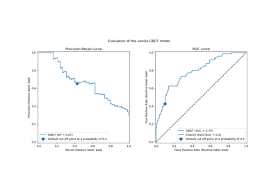
Our predictive model succeeds to grasp the relationship between the data and the target. The training and testing scores are close to each other, meaning that our predictive model is not overfitting. We can also observe that the balanced accuracy is lower than the accuracy, due to the class imbalance previously mentioned.
For this classifier, we let the decision threshold, used convert the probability of the positive class into a class prediction, to its default value: 0.5. However, this threshold might not be optimal. If our interest is to maximize the balanced accuracy, we should select another threshold that would maximize this metric.
The TunedThresholdClassifierCV meta-estimator allows
to tune the decision threshold of a classifier given a metric of interest.
Tuning the decision threshold
We create a TunedThresholdClassifierCV and
configure it to maximize the balanced accuracy. We evaluate the model using the same
cross-validation strategy as previously.
from sklearn.model_selection import TunedThresholdClassifierCV

tuned_model = TunedThresholdClassifierCV(estimator=model, scoring="balanced_accuracy")
cv_results_tuned_model = pd.DataFrame(
    cross_validate(
        tuned_model,
        data,
        target,
        scoring=scoring,
        cv=cv,
        return_train_score=True,
        return_estimator=True,
    )
)
cv_results_tuned_model[cv_scores].aggregate(["mean", "std"]).T
In comparison with the vanilla model, we observe that the balanced accuracy score increased. Of course, it comes at the cost of a lower accuracy score. It means that our model is now more sensitive to the positive class but makes more mistakes on the negative class.
However, it is important to note that this tuned predictive model is internally the same model as the vanilla model: they have the same fitted coefficients.
import matplotlib.pyplot as plt

vanilla_model_coef = pd.DataFrame(
    [est[-1].coef_.ravel() for est in cv_results_vanilla_model["estimator"]],
    columns=diabetes.feature_names,
)
tuned_model_coef = pd.DataFrame(
    [est.estimator_[-1].coef_.ravel() for est in cv_results_tuned_model["estimator"]],
    columns=diabetes.feature_names,
)

fig, ax = plt.subplots(ncols=2, figsize=(12, 4), sharex=True, sharey=True)
vanilla_model_coef.boxplot(ax=ax[0])
ax[0].set_ylabel("Coefficient value")
ax[0].set_title("Vanilla model")
tuned_model_coef.boxplot(ax=ax[1])
ax[1].set_title("Tuned model")
_ = fig.suptitle("Coefficients of the predictive models")

Only the decision threshold of each model was changed during the cross-validation.
decision_threshold = pd.Series(
    [est.best_threshold_ for est in cv_results_tuned_model["estimator"]],
)
ax = decision_threshold.plot.kde()
ax.axvline(
    decision_threshold.mean(),
    color="k",
    linestyle="--",
    label=f"Mean decision threshold: {decision_threshold.mean():.2f}",
)
ax.set_xlabel("Decision threshold")
ax.legend(loc="upper right")
_ = ax.set_title(
    "Distribution of the decision threshold \nacross different cross-validation folds"
)

In average, a decision threshold around 0.32 maximizes the balanced accuracy, which is different from the default decision threshold of 0.5. Thus tuning the decision threshold is particularly important when the output of the predictive model is used to make decisions. Besides, the metric used to tune the decision threshold should be chosen carefully. Here, we used the balanced accuracy but it might not be the most appropriate metric for the problem at hand. The choice of the “right” metric is usually problem-dependent and might require some domain knowledge. Refer to the example entitled, Post-tuning the decision threshold for cost-sensitive learning, for more details.
Total running time of the script: (0 minutes 31.738 seconds)
Related examples
Post-tuning the decision threshold for cost-sensitive learning
Recursive feature elimination with cross-validation
Class Likelihood Ratios to measure classification performance